Not long after its inception at Motorola in the mid 1980’s, Six Sigma’s practitioners began to realize that there is often a practical limit to how much existing products or processes can be improved. This limit is sometimes referred to as the “five sigma barrier” because it is in this region of process performance that the financial gain of further improvement is frequently outweighed by the cost of implementation. At approximately 233 defects per million (dpm), a five sigma process is well above average when compared to most manufacturing processes.
Consequently, improving an “average” process to this level of performance will typically yield significant financial benefit. Nevertheless, a 5 sigma process may not be sufficient for many critical process steps. In fact, in the pharmaceutical industry, even the “world class” six sigma standard (3.4 dpm) is inadequate with respect to the occurrence of some critical defects. Given the limitations of the 5 sigma barrier, how can we achieve an appropriate level of process performance while maintaining a competitive operating cost?
Fortunately, the Six Sigma pioneers at Motorola, General Electric and other companies realized that the five sigma barrier often occurs as a result of product features which are an inherent part of the product design. If the design team did not perform a sufficient number of studies to develop a thorough understanding of the product or process, it is possible that they may have inadvertently designed limitations, or possibly even quality issues, directly into the product. Although the adverse affects of these design issues were certainly unintentional, often these problems cannot be remedied unless we completely redesign the existing product. The cost of redesign is often the road block which results in the 5 sigma barrier.
It was also recognized by these pioneers, that even if these design flaws were identified prior to product launch, the later in the development cycle that they were discovered, the more costly they became to correct. While this fact is probably true for all kinds of products, it is particularly true in the pharmaceutical industry. Although Scale-Up and Post Approval Changes (SUPAC) guidelines provide direction regarding regulatory requirements to support post approval formulation modifications, changes to process parameters and other registered details; in some cases the cost of these studies can become an insurmountable barrier which may prevent a company from implementing the improvements. Unfortunately, the penalty for inaction is often equally daunting as the product could be subject to frequent batch rejections, extensive investigative testing and possibly even a product recall. All of these events have a significant financial cost but they could also potentially cause irreparable damage to brand and corporate reputation as well. Certainly, as in other industries, the pharmaceutical industry has a well vested interest in developing quality products which require little or no modification after registration and commercial launch. How can we identify and avoid these design flaws? In other words, how do we make sure that we “get it right the first time” without spending extraordinary amounts of time and money in development?
Recognition of the costs associated with poor product design led early Six Sigma practitioners to the development of an additional set of tools and techniques which became known as Design for Six Sigma (DfSS). Among the primary objectives of DfSS is the identification of these shortcomings early in the product development cycle with the intent to eliminate them before the cost of change becomes overwhelming.
Conventional Six Sigma uses various methods to identify and eliminate the root causes of variation which adversely affect the performance of existing products and processes. Essentially, it helps us to improve what we are already doing by ensuring we do it more consistently and with fewer mistakes. As its name implies, the focus of DfSS is further upstream in the product lifecycle. It is applied during the early stages of concept development and the design of a new product or, alternatively, during the redesign of an existing product.
The primary goals of DfSS are to clearly understand the customers requirements and to design a product which is highly capable of meeting or exceeding those requirements. Additionally, DfSS provides the tools and a structured approach to efficiently create these new products by helping to minimize effort, time and costs required to design and eventually manufacture the new product on an on-going basis. The fundamental premise behind DfSS is that in order to effectively achieve these goals, we must thoroughly understand the process and product such that critical material and process parameters are identified and appropriately controlled. The DfSS toolbox has a wide variety of tools and methods, some of which are shared with conventional Six Sigma, to help achieve these goals.
The savvy reader has probably already recognized that the primary objectives and principles underpinning DfSS are completely aligned with the fundamental philosophy of QbD. Guidance documents published by ICH, FDA and other regulatory bodies frequently refer to the need for pharmaceutical R&D teams to develop an “enhanced” level of process knowledge using sound scientific methods and experimentation. This is why these two approaches compliment each other so well.
This paper will take a closer look at this overlap between Design for Six Sigma and Quality by Design, as well as introduce DfSS tools—including Monte Carlo Simulation, Parameter (robust) Design, and Tolerance Allocation—which can also be used to support a QbD program.
Inputs and Outputs
According to ICH Q8, “The aim of pharmaceutical development is to design a quality product and its manufacturing process to consistently deliver the intended performance of the product.” This objective can be attained by using an “empirical approach or a more systematic approach to product development.” DfSS and QbD are very much focused on the latter. Both philosophies are founded upon the definition and understanding of the product, its performance requirements, and the processes by which it is manufactured and packaged.
In very general terms, every process is a blending together of inputs to produce some desired output. Typically, the quality or performance of the product and process is determined by measuring one or more properties of the output. A process input is a factor that if it is intentionally changed, or if it is not appropriately controlled, it will have an affect on one or more of the process output performance measures. Inputs typically include: equipment parameters, raw material properties, operators as well as the policies and procedures they follow, measurement systems, environmental conditions and potentially many other important factors.
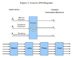
The generic Input – Process – Output (IPO) diagram in Figure 1A, illustrates, at a high level, the inputs (X’s) related to one or more process outputs (Y’s). The inputs listed in Figure 1A are very broad categories. In actual practice, the development team will have to identify very specific inputs. Additionally, as illustrated in Figure 1B, most production processes are sufficiently complex that it will be necessary to sub-divide the process into major sequential steps. Typically, at least some of the outputs from one process step will become the inputs to the subsequent step. Often, particularly in early development, the team will be monitoring a wide variety of outputs at each stage, up to and including the performance of the finished product. Ultimately, our goal is to understand the relationships between the critical inputs and outputs of each step.
Figure 1A: IPO diagrams illustrate input factors (X1, X2, X3….. Xn) related to the quality or performance measures of interest (Y1, Y2, Y3…. Yn). The inputs listed as examples in this diagram are very broad generic categories. In actual practice, the development team will have to identify specific inputs and outputs for each process step.
Figure 1B: Due to the sequential nature of most processes, it is typical that some of the inputs from one process step are related to and dependent upon the outputs of the preceding step. Given the complexity of most pharmaceutical processes, it is likely that it will be necessary to evaluate the inputs and outputs of each major process step separately.
One of the first tasks to be completed when developing a new product is to understand the performance requirements of the finished product. Although in early development we often do not have well defined specifications, once all of the performance measures have been at least generally identified, it is possible to start listing all of the inputs that may affect the outputs of interest. As suggested in ICH Q8 (R1), using prior knowledge of similar products and the results of preliminary experimentation, the development team could perform a brainstorming exercise to create fishbone diagrams listing all known and potential factors which could impact each of the outputs. This initial effort should result in an exhaustive list of inputs on the basis of current knowledge. However, it is likely that this list will grow and evolve as the team learns more about the product and process.
As also suggested by ICH Q8 (R1), a Failure Mode and Effects Analysis (FMEA) might also be used to rank the many factors which are on the various fishbone diagrams. As indicated in several of the ICH guidance documents and other regulatory publications, FMEA and other risk management tools should be applied at all stages of product development so that appropriate controls can be implemented as more is learned about the product and process. Depending on which stage of the development cycle the team is working on, there are several different approaches which could be applied when using the FMEA tool. Two of these, which could be used in the early stages of development, include a step by step review of the process and a component review of the formulation. When using the former approach, the team must identify the intended function of each process step. Next, the team must ask what could go wrong with that step that could impair or prevent it from delivering the intended function. Similarly, using the second approach, after listing every component of the formulation, the team must ask, what is the intended purpose of each component and how could it fail to perform that function. The results of these exercises will be rated in terms of their severity, likelihood of occurrence, and probability of escaped detection. The product of these individual ratings provides a rank ordered list using the Risk Priority Number (RPN). Like the fishbone diagrams, an FMEA is a living document which should be revisited, revised and augmented multiple times during the development cycle.
Finding the “Vital Few”
DfSS, like QbD, is based upon the development of an understanding of the relationship between specific input parameters and the performance of the finished product. After completing the initial versions of the fishbone diagrams and FMEA, the team will have an extensive list of potentially important factors. How does it determine which ones are actually “critical to quality” with respect to the performance of the finished product?
On the basis of the results of the FMEA exercise, prior knowledge and preliminary experimentation, the team should be able to create a shorter list. However, they will probably not yet have enough knowledge or data to narrow the list to what Dr. Joseph Juran referred to as the “vital few among the trivial many.” Hence, additional tools are needed.
A statistically designed experiment, often referred to as a Design of Experiments (DoE), is one way to efficiently and scientifically narrow the list of factors. There are many different designs which could be used for this purpose, each with their own pros and cons.
At a preliminary screening stage, it is best to test the maximum number of factors while performing the fewest possible experiments. For example, a Taguchi L12 design will allow us to evaluate the relative importance of up to 11 factors using just 12 experimental runs. One of the limitations of this design is that, although it provides information regarding the relative importance of the individual factors, it does not give information on possible interactions between those factors. Nonetheless, it is a good first step towards ranking factors under investigation.
Transfer Function
Once the list of “most important” factors has been reduced to a manageable size, other DoE designs may be used to provide information on some or all factor interactions. Full or fractional factorial designs can be used to produce an empirical model which mathematically describes the relationship between the inputs and the output(s) of interest. In DfSS jargon, this mathematical prediction equation is known as a transfer function.
The transfer function is an extremely valuable piece of process knowledge. Given specific values for the inputs, it can provide a means to predict the average value of the output(s). Conversely, if the desired value or a specification range of the output is known, it can be used to identify optimum operational and material parameters to achieve the desired average response.
Almost always, the team is interested in more than one output. Fortunately, it is possible collect data on multiple outputs for each experimental run, and then use all of this information to predict the best conditions that satisfy the specifications for each of the outputs. This technique is known as multiple response optimization.
Unfortunately, there is no guarantee that a perfect solution exists. Although it is possible to mathematically explore the experimental space described by the transfer functions, there may or may not be a location (the design space) that will consistently satisfy all of the specifications at the same time. If the development team finds itself in this situation, at least they identified this problem relatively quickly and efficiently. Additionally, much of the knowledge they have gained on this first attempt can help them to regroup and find solutions later in development.
Monte Carlo Simulation
A wide variety of other DfSS statistical tools can be applied using the transfer function. One of these tools is Monte Carlo Simulation (MCS), sometimes referred to as Expected Value Analysis (EVA). Among other things, MCS can be used to predict process capability—i.e., it can predict how well the process is expected to perform relative to its specification(s).
In many cases, applying the average values of inputs to the transfer function will predict the average value of the output(s). Unfortunately, this approach does not consider the fact that most inputs are not perfectly constant—that is, they are not always going to be equal to the average value. Inputs may vary from one day to the next, from lot to lot or even operator to operator. Although controls are often implemented to hold these factors constant or within a specified range, the ability to do so is sometimes limited by technology or cost. The advantage MCS offers is that, if the long-term distribution parameters (e.g., the mean and standard deviation of a normally distributed factor) can be estimated for each critical input, these estimates can be applied to the transfer function and used to predict what the expected distribution of the output(s) will be over the long term, across many batches.
Figure 2 represents an Input-Process-Output (IPO) diagram which indicates that the process inputs have three different distributions. In this example, inputs X1, X2, and X3 appear to be normally, exponentially, and uniformly distributed. The MCS will “randomly draw” one value from each of these distributions and apply those values to the transfer function to generate a single result for the predicted value of the output(s). It will repeat this process as many as one million times. The histogram of the resulting values will provide an estimate of the output distribution which can then be compared to the specifications for that performance metric.
Monte Carlo Simulation (MCS) applies the characteristics of known or estimated input distributions to the transfer function of each output in order to produce an estimate of the distribution of that output. If output specifications have been developed or proposed, process capability and the associated defect rate (dpm) can also be predicted.
The ability to predict process output capability not only allows the team to estimate the defect rate for the intermediate or finished product which is under investigation, but it also allows a direct comparison of the relative performance of various formulation options, processes or products which may be under consideration in the early stages of development.
Process Robustness and Specifications
Any process should be “robust” to the variation of process inputs which are difficult or expensive to control. Let’s say the particle size distribution (PSD) of a micronized active pharmaceutical ingredient (API) is difficult to control. If PSD is an important factor with respect to dosage uniformity, rather than tightening the specification and perhaps paying a premium to the supplier, it would be preferable to find operational conditions which are tolerant of this variation; that is, teams can identify conditions under which the dosage uniformity is relatively unaffected even in the presence of the PSD variation.
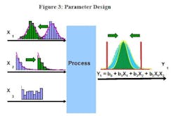
Several DoE techniques can help make a process robust to variation in certain input variables, though many of these become difficult and cumbersome to apply when dealing with multiple responses. Another DfSS tool, Parameter Design, explores the experimental space looking for regions which make the process relatively insensitive to the known variation of the inputs. Parameter Design shifts the average response of the various inputs and evaluates the effect on the output distributions. If successful, it will find a combination of average input settings which achieve the same average output response, but with less variation around that average.
Parameter Design explores the experimental space looking for regions which make the process tolerant of the known variation of some difficult to control process inputs. In this example, the average value of X1 has been reduced and the average value of X2 has been increased (input distributions have been shifted from the blue to the green histograms). Effectively the variability of the inputs and the average response remain the same, but the variation around the average response has been significantly reduced (green output histogram) resulting in a process which is tolerant (robust) to the variation of the inputs. To simplify the example, only one response has been used in this illustration, but multiple responses can be evaluated simultaneously.
If the team is not able to find any robust regions within the design space (they may not exist), they may tighten the input specifications to reduce the output variation. Intuitively, many process scientists and engineers believe that tightening the specification of an input will reduce the output defect level, and in fact this is often true. However, what is often not intuitive is the ability to identify which factors will have the greatest impact and to what degree specifications need to be tightened. Typically, asking suppliers or the manufacturing team to meet a tighter specification on a raw material attribute, or an operating parameter, will result in an increase of operational cost. Consequently, it’s important to prevent a situation where input specifications are tightened “just to be sure.”
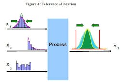
Tolerance Allocation allows the team to understand the effect of changing the variation of each input on the variation of the output(s). In contrast to Parameter Design which shifts process averages, Tolerance Allocation will evaluate the effects of individually increasing and decreasing the standard deviations of each of the input factors. It will estimate the expected number of defects per million (dpm) under each of these trial conditions. The resulting matrix gives the team the knowledge required to set appropriate specifications for each input.
If lucky, the team might be able to identify opportunities to relax some of the current specifications with little or no negative impact on quality metrics. These opportunities could possibly even offset the cost of tightening other specifications. The big advantage of Tolerance Allocation is that it provides the opportunity to make educated decisions regarding where best to invest in tightening a specification.
Tolerance Allocation evaluates the effect of individually increasing and decreasing the standard deviation of process inputs. In this example, reducing the variation of X1 (the green dashed line represents the distribution resulting from a tightened specification) has significantly reduced the variation of the output (green output histogram). This approach allows the team to identify which inputs will have the greatest impact on the output variation and thereby helps to balance cost-benefit trade-offs and set appropriate specifications for each of the process inputs.
Conclusions
DfSS and QbD share a common philosophy which is based upon the principle that employing a systematic and structured approach to product development will increase the amount of process knowledge the development team obtains, thereby allowing them to make better decisions and increase the probability of successfully developing a quality product which will consistently perform as intended.
In addition to the tools typically associated with QbD, DfSS provides other techniques which can further enhance the development team’s knowledge. The experimental transfer functions which the team generates are simply process models which can be used to better understand, optimize and predict the expected performance of the process or product. As with any model, experimentation must also be performed to confirm those predictions. Nonetheless, these equations will help the team to accelerate their progress along the development path by focusing their efforts on the best options to be investigated.
While these tools are not a substitute for development expertise, they are a potent supplement which will help to maximize the benefit of the knowledge and experience the team already possesses. When compared dollar for dollar and data point for data point, these tools will provide more information and help the team avoid the quagmire of the “shot gun” approach in which a potentially endless string of “what if” scenarios are evaluated. There is no avoiding the fact that pharmaceutical development requires a huge investment of resources and funding. DfSS and QbD can help us to ensure we maximize the return on those investments, not only during product development, but also for years to come after product launch.
About the Author
Murray Adams is a certified Master Black Belt and the Managing Director of Operational Excellence, a consulting company that provides Six Sigma and DfSS analysis, training, and coaching to clients in a wide variety of industries. He can be reached at [email protected].
Suggested References
Peterson, J. J. What Your ICH Q8 Design Space Needs: A Multivariate Predictive Distribution. http://www.pharmaqbd.com/node/453
Kiemele, M.J. and Reagan, L.A. Design for Six Sigma: The Tool Guide for Practitioners, CTQ Media, Washington (2008).
Chowdhury, S. Design for Six Sigma: The Revolutionary Process for Achieving Extraordinary Profits. Dearborn Trade Publishing, Chicago (2002).
