Reduce Calibration Costs and Improve Sensor Integrity through Redundancy and Statistical Analysis
There exists a market need, dictated by the FDA, to maintain the accuracy of sensors in a validated pharmaceutical process. Today, this is achieved by: 1) installing certified instruments; and 2) maintaining a costly routine calibration protocol.
FDAs process analytical technology (PAT) initiative has opened the door to a fresh look at applying technology for productivity improvements in the pharmaceutical industry. The application of online, real-time analytical instruments was the first trend of the PAT initiative. This paper addresses another aspect for cGMP data integrity. It takes a novel approach to maintaining data integrity through the use of redundancy and statistical analysis. The result is reduced calibration cost, increased data integrity and reduced off-spec uncertainty.
Today, pharmaceutical companies write elaborate calibration protocols that are consistent (and sometimes overly compliant) with FDA cGMP guidelines to maintain the reported process value integrity. This can result in extremely high cost for compliance with only a minimum ROI for improved productivity or product quality. For example, one pharmaceutical site in New Jersey conducts about 2,900 calibrations per month. Of those, about 500 are demand maintenance where the instrument has clearly failed as evidenced by a lack of signal or a digital diagnostic (catastrophic failures). The remaining 2,400 calibrations are scheduled per protocol. Of these, only about 400 calibrations find the instrument out of calibration. The majority, about 2,000 calibrations per month, find the instrument still working properly. Those at other pharmaceutical manufacturing facilities can check orders from the metrology department and obtain the exact ratio for their facility, and might be surprised to find similar numbers.
This paper describes an alternate instrument scheme consisting of the use of redundant sensors and statistical analysis to avoid unnecessary calibrations and to detect sensors that are starting to drift before they go out of calibration.
The new approach is:
- To install two dissimilar instruments to sense the critical (cGMP) value
- To track their relative consistency via a statistical control chart
- Upon detection of the two values drifting apart, to determine which instrument is drifting as a function of the relative change in the individual instruments change in standard deviation.
- To use the process alarm management system to alarm the operator that
a. the sensors are drifting apart
b. most likely, the faulty instrument is the one with the changing standard deviation
If there are no alarms:
- Both instruments are tracking
- The operator and control programs can assume there is high data integrity
- There is no need for routine calibration.
The economic justifications of this approach are:
- Hard savings: Cost of second instrument versus periodic calibrations
- Soft savings: Cost of auditing product quality for everything that was affected by the failed instrument since its last calibration
Figure 1: There is a need and hidden cost to evaluate all product and performance that may have been affected by the undetected failure of a cGMP instrument.
In light of the high frequency and high cost of performing calibrations in a validated environment and the downside risk and cost of quality issues, the potential savings can be huge. Therefore, the life cycle cost can warrant the increased initial investment in a second instrument and the real-time statistical analysis of the instrument pair.
Calibration Basics
Let us begin by establishing a base level of understanding of instrumentation calibration.
Precise, dependable process values are vital to an optimum control scheme and, in some cases, they are mandated by compliance regulation. Precision starts with the selection and installation of the analog sensor while the integrity of the reported process value is maintained by routine calibration throughout the life of the instrument.
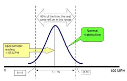
When you specify a general purpose instrument, it has a stated accuracyfor example, +/- 1% of actual reading. In the fine print, that means that the vendor states that the reading of the instrument will be within 1% of reality 95% of the time (certainty).
For example, if a speedometer indicates that you are traveling at 55 mph and the automobile manufacturer installed a +/- 1% speedometer, then you do not know exactly how fast you are going but there is a 95% probability that it is somewhere between 54.45 and 55.55 mph. See Figure 2.
Figure 2: Accuracy of a speedometer
There are two reasons why this situation is acceptable when 5% of the time the instrument is probably reporting a value that is more than 1% inaccurate:
- Cost / value tradeoff: The inaccuracy will not effect production or quality
- The next reading has a 95% chance of being +/- 1% of reality, therefore placing it within specs
If you need to improve the accuracy of the values, you can specify:
Once installed, periodically re-calibrating the instrument based on drift specification provided by the instrument vendor, owner/operator philosophy or industry guideline GMP will assure the integrity of the value. Although periodic calibration is the conventional solution, the 2,400 scheduled calibrations referenced above present two economic hardships:
- The 2,000 calibrations that simply verify that the instruments are still operating within specifications are pure non-ROI cost
- The 400 that are out of spec create an even more troublesome problem. If the instruments process value is critical enough to be a validated instrument that requires periodic calibration, then what happens when it is discovered to be out of calibration? By protocol, must a review of all products that have been manufactured since the last known good calibration occur? Probably yes, because if the answer is no it begs the question as to why this instrument was considered a validated instrument. If the instrument is only slightly out of calibration but still within the product/process requirements, the review may be trivial. If it is seriously out of calibration, a comprehensive quality audit or product recall may be mandated by protocol.
Unavailability vs. Integrity
We recognize the distinction between catastrophic failure resulting in unavailability and loss of integrity. A catastrophic failure is one in which the instrument does not perform at all, while a loss of integrity failure is one in which the instrument does not perform correctly. A catastrophic instrument failure is easy to detect because there is no signal coming from the instrument or, in the case of an intelligent device, there is an ominous diagnostic message. A catastrophic failure renders the instrument unavailable.
A loss-of-integrity instrument failure is more esoteric because there is a signal but it is not accurate. Moreover, it is insidious because there is no inherent way to recognize that the reported value is inaccurate. Unlike most man-made devices, an instrument may not show symptoms of degradation before it fails catastrophically. An automobile will run rough or make a noise before it breaks down. A degrading instrument will provide you a value; you have no inherent way to recognize that it has drifted out of specifications. It will appear to be operating properly. There is no equivalent perception of rough-running automobile.
If the value is so critical that process management cannot operate without it, then conventional wisdom suggests the installation of two instruments for increased availability. However, the primary flaw in conventional wisdom is that a second instrument only increases availability and minimizes the probability of a catastrophic failure (If one breaks, use the other value).
Unfortunately, the addition of a second instrument does not improve the data integrity. In fact, redundant instruments expose the issue of data integrity! What happens if the two instruments are not communicating the same value? How far apart can the values drift before remedial action is initiated? Do you trust one instrument and not the other while the remedial action is being performed? Which signal can be trusted? Availability does not address quality or performance.
For sensors, data integrity is the measure of their performance. So what should you do when the reported values from two instruments that are supposed to be sensing the same thing differ? If they are close enough, you can use either value, A or B, or both, (A + B) / 2.
The question is what is close enough? Some prefer a very liberal tolerance such as the sum of the stated accuracies of the two instrumentsi.e., 1% + 1% = 2%. Most prefer their root meanthat is, square root of (1%² + 1%²) = 1.4%.
If they are too far apart:
- Use A or B or (A + B) / 2 anyway or,
- Use the last value or,
- Use the lower value or,
- Use the higher value or,
- Stop everything and call maintenance.
Breakthrough
Advancements in computer power and statistical analysis tools now make it possible to make a major breakthrough and solve the reliability problem. The solution is:
- Install two different types of instruments to measure the process variable
- Analyze their signals to verify they are properly tracking each other
- Alarm operations and maintenance when they begin to drift apart
- Identify the suspected failing instrument.
The use of dissimilar instruments reduces the possibility of common cause failure that may result if identical instruments were damaged by a process anomaly and happened to fail in a similar fashion.
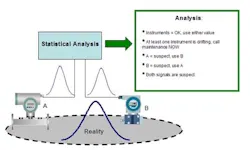
The analysis would provide a constant level of assurance that the process value has data integrity. Its analysis will constantly verify the two instruments are not drifting apart. Since they are dissimilar instruments, it is highly unlikely that they would go out of calibration at the same time, in the same direction and at the same rate as to avoid statistical recognition that they are drifting.
Figure 3: Statistical Analysis Results
If the two signals begin to drift apart, the analysis will alarm the situation.
Finally, the analysis engine will then analyze the historical data and identify which signal is behaving differently. The assumption is only one instrument will fail at a time. Therefore, analysis of historical data will determine which instruments performance is changing.
If both are changing, then there has probably been a change in the process, and the entire process needs to be examined. This is a vital and new insight that previous, single-sensor topographies were unable to provide. It can dramatically:
Increase:
o the overall integrity of the control system
o the quality of production
o the productivity of the metrology lab
Decrease:
o the mean time to repair (MTTR) of failing sensors
o the cost of remedial quality assurance reviews that are mandated when a critical (validated) sensor is discovered to have failed some time in the past.
The breakthrough is the fact that the statistical method will detect very slight shifts in the two instrument signals long before an instrument violates a hard alarm limit, such as the square root of the sum of the accuracies. This method of real-time calibrating and alarming on the slightest statistically significant deviation renders conventional periodic calibration practices obsolete. We can reduce the cost of unnecessary periodic calibrations caused by the discovery of a critical instrument out of calibration during a periodic calibrationby declaring the calibration protocol to calibrate whenever (and only when) the statistical alarm indicates a deviation in values, which minimizes the impact on production and product quality.
Proof of Concept
The proof of concept is a series of alpha level tests. A 1,000-sample test data using random numbers to simulate sensor noise and biasing the noise to simulate drift was created using Microsoft Excel. The data was then analyzed in a statistical tool, MiniTab.
Sensor A values equal a random number (0 to 1.0) added to the base number 99.5. This simulates a field signal of 100 +/- .5. That is a sensor reading 100 +/- .5%. The random number simulates the noise or uncertainty of an instrument that is designed to provide a value that is +/- .5% accurate.
Sensor B is identically structured but uses a different set of random numbers.
Results indicate that statistical control charts and F-test calculations identify drift and the suspect sensor much faster than conventional detection. Typically, in two-sensor configurations, the alarm limit to recognize two sensors are reading different values is set at the root mean square of the stated accuracies of the two instruments.
Preliminary research found the statistical method is more sensitive. Drift can be detected in about 1/3 the movement, thus giving operations and maintenance even more time to respond to the drifting instrument before it goes officially out-of-calibration and triggers other remedial actions that are dictated by protocol to assure product quality.
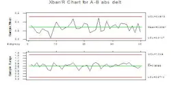
First test evaluates the comparison of sensor A and sensor B. The first control chart (Figure 4) evaluates the absolute value of the differences between Sensor A and Sensor B. 1,000 pairs of values in subgroup size = 25. This simulates capturing pairs of sensor readings at some convenient periodsay, once a minute, an hour, a fortnightand executing an Xbar control chart on the last 1,000 readings.
Figure 4: Statistical control chart of the delta between pairs of Sensor A and Sensor B simultaneous readings. No statistical alarms are detected.
The control chart finds the sensors in statistical control. There are no alarms, as expected, because the simulated signal noise is the result of a random number generator and we have not yet injected any error/bias/instrument drift.
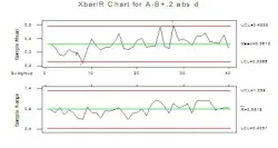
The second test evaluates the 1,000 pairs of data with bias added to Sensor B. The Sensor B oldest 500 values are identical to the first test. The Sensor B most recent 500 values have been altered by adding 20% of the random number to the sensor's value. That is Sensor B values for 1 to 500 are 99.5 + random B. Sensor B values from 501 to 1000 are 99.5 + random B + .2 * random B. This simulates an instrument starting to become erratic.
The second control chart (Figure 5) finds the absolute value of the differences between Sensor A and failing Sensor B out of statistical control. You will notice that there are alarms, as expected, because the simulated signal noise has been slightly amplified to simulate that Sensor B is becoming a little erratic and may be beginning to drift.
Figure 5: Statistical alarms begin to show up when the simulated noise (randomness) in Sensor B amplified by 20%.
The red numbers superimposed on the chart are the statistical alarms. The numbers represent the following alarm criteria:
1 = One point more than 3 sigma from center line
2 = Nine points in a row on same side of center line
3 = Six points in a row, all increasing or all decreasing
4 = Fourteen points in a row, alternating up and down
5 = Two out of three points more than 2 sigma from center line (same side)
6 = Four out of five points more than 1 sigma from center line (same side)
7 = Fifteen points in a row within 1 sigma of center line (either side)
8 = Eight points in a row more than 1 sigma from center line (either side)
Notice also the sensitivity. With conventional dual-instrument configurations, the alarm limits are set at +/- root mean squared (RMS) of the sum of their stated accuracies (i.e. square root of (0.5%² + 0.5%²) = 0.707%). The mean difference is statistically about half that at, in this data set, 0.338%. The Xbar/R Chart detected drift when the mean difference between the Sensor A values and the Sensor B values drifted by a mere .023%. In other words, the control chart detected a change in the comparable performance of the two sensors when the noise of one instrument grew by only 20%.
Both instruments are still tracking one another and well within the conventional delta of 0.707% but one is beginning to become erratic. It is now time to calibrate Sensor B. Meanwhile, the system has maintained its integrity.
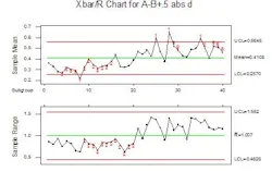
Now we repeat the test with injecting error equal to 50% (i.e., we let the random number that is simulating noise in Sensor B have an increase of 50% in amplitude for the newest 500 instrument readings).
Figure 6: Statistical alarms are clearly present when the simulated noise (randomness) in Sensor B amplified by 50%.
Notice that the mean value between the two instrument readings is still only 0.4108 but clearly the control chart has correctly detected an increased erratic behavior.
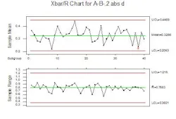
The next control chart (Figure 7) simulates an instrument starting to lose sensitivity. This could happen if the instrument has fouled, become sluggish or is about to go comatose.
It charts the absolute value of the differences between Sensor A and failing Sensor B. Again, sensor Bs oldest 500 values are identical to the first test. Sensor Bs most recent 500 values have been altered by subtracting 20% of the random number to the sensor's value. I.E. Sensor B values for 1 to 500 are 99.5 + random B. Sensor B values from 501 to 1000 are 99.5 + random B - .2 * random B.
Figure 7: A statistical alarm is clearly present when a drop in noise is simulated in Sensor B by attenuating the random component by 20%.
Notice that a drop in the responsiveness (randomness) of the signals by a mere 20% can be detected.
You will notice that the there is at least one alarm (as expected) because the simulated signal noise has diminished to simulate that Sensor B is losing sensitivitybecoming becoming flatlined.
Again, notice the sensitivity. The Xbar/R Chart detected drift when the mean difference between the Sensor A values and the Sensor B values closed by a mere 0.012%. In other words, the control chart detected a change in the comparable performance of the two sensors when the noise of one instrument decreased by only 20%. Both instruments are still within calibration, but one is beginning to lose its integrity.
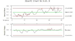
If we eliminate 90% of the noise from sensor B, simulating a non-responsive, flatline, comatose instrument, we get the following. See Figure 8.
Figure 8: Statistical alarms are extensive when Sensor B loses sensitivity.
Again, the mean difference has not drifted too far apart but the statistical analysis has recognized the lack of responsiveness. It is now time to calibrate.
Sensor reliability and data integrity is assured as long as the pairs of sensors continue to pass the statistical analysis review. When they fail, an alarm generated by the real-time control chart can be triggered through the process control alarm management system. Thus, there is no need to perform periodic calibrations.
However, when statistical analysis detects an emerging problem, it is necessary to continue operations while the problem is remedied. Further statistical analysis can also be used to identify the most likely cause of the alarm. With this information, operations can continue and the MTTR can be shortened.
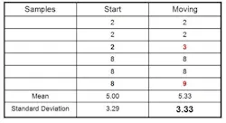
Figure 9 shows a very interesting statistical phenomenon.
Figure 9: Shifting mean is seen in change in variance
When a sample is shifting from one mean to another, the variance increases during the transition period. In this example, two data, a 2 and an 8 shifted a mere one unit to the right to become a 3 and a 9. The result is that the mean shifted to the right from 5.0 to 5.33 and the standard deviation also shifted up from 3.29 to 3.33. See Figure 10.
Figure 10: Shift in variance
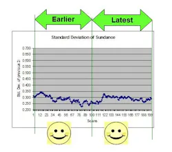
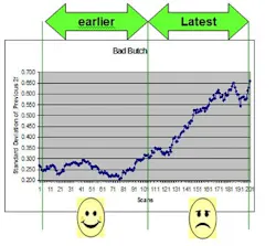
We use this shift to detect drift. The sample values from the two instruments will go up and down with changes in the real-world value that is being sensed. Therefore, the actual mean value is of little consequence to the task of detecting instrument drift.
The key factor is the variance. It should maintain statistical consistency over time. Both instruments means and standard derivations should track. When their means drift too far apart as detected by the control chart test, then we look at the behavior of the standard deviation to determine which instrument is behaving differently. The one that has a significant change in its variance (up or down) is suspect. If it has gained variance relative to its past, it is becoming unstable. If it has lost variance, it is becoming insensitive or has fouled. In either case, the sensor that has a significant change in its variance over time while the other sensor has not had a significant change. This sensor is suspect and the probable specific cause of the delta in means between the two sensors.
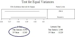
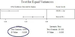
The next series of tests determine which sensor is experiencing a failure using an F-test. The hypothesis is that the failing sensor can be detected by a change in the variance of the sample. This technique subgroups the sample into groups of 25 and calculates each subgroups variances. Then the variances of the oldest 500 samples are compared against the newest 500 samples. The sensor that is not experiencing change will pass the F-test while the sensor that is experiencing a change (more variation in its readings) will fail the F-Test.
The first test compares the variance of old A to recent A. The F-Test p-Value of .560 (>.05) indicates that the variances are equal.
Figure 11: F-Test on Sensor A.
The second test compares the variance of old B to recent B. The F-Test p-Value of .00 (>.05) indicates that the variances are different.
Figure 12: F-Test on Sensor B
Since A does not seem to be changing and B does seem to be changing, we can issue an advisory that declares B is suspect.
Summary
In conclusion, the FDA has been encouraging the use of statistics and other technologies as part of the PAT initiative. This paper has demonstrated that we can dramatically improve the data integrity of the critical instrument signals through redundancy and statistical analysis. In fact, one could argue that if statistical calibration is done in real-time, then costly periodic manual calibration is no longer necessary.
Significant improvements in data integrity will reduce the life cycle cost of the instrumentation and calibration functions and minimize the downside risk of poor quality or lost production caused by faulty instrumentation.
Two Other Notes:
This paper offers a hypothesis and a proof of concept. Several other statistical tools such as Pair-t test and Gage R&R were tested with varying degrees of robustness. There is no perfect choice of tool. Likewise the selection of a sample size of 1,000 and subgroups of 25 was arbitrary and remain open research topics.
Finally, the use of statistics to detect drift and the need for instrument calibration may have many other applications outside of the pharmaceutical industry. In particular, any two or more devices that need to track performance such as propellers, boilers or transformers can possibly be monitored and imbalances detected long before the imbalance damages the equipment.
One other very intriguing application is the reduction of instrumentation in a safety system. With the statistics tool able to detect which instrument is failing, a two-instruments-plus-statistical-tool configuration will provide the same coverage as a two-out-of-three configuration. Both a two-instruments-plus-statistical-tool configuration and a twoout-of-three instrument configuration will detect a drifting analog value. Neither configuration can absolutely resolve a second failure. In essence, the two-plus-statistical-tool is replacing the third instrument with a software package. Since a software package can be applied to multiple loops and requires less maintenance and energy to operate, there can be tremendous life cycle cost savings opportunity.
Bibliographical References
Measurement Uncertainty: Methods and Applications by Ronald H. Dieck, Third Edition, Instrument, Systems, and Automation Society, 2002
Practical Statistics by Example Using Microsoft Excel and Minitab by Terry Sincich, David Levine, David Stephan, Second Edition, Prentice-Hall, 2002
Economics of Control Improvement by Paul G. Friedmann, Instrument, Systems, and Automation Society, 1995
Design for Six Sigma by Subir Chowdhury, Dearborn Trade Publishing, a Kaplan Professional Company, 2002
System Availability Evaluation version V1, revision R2, May 5, 2005, by Iwan van Beurden, a white paper by Exida
About the Author
Dan Collins is the Manager of DCS Solution Partner Program for Siemens Energy & Automation. Dan has more than 30 years of industrial instrumentation and controls experience with previous assignments in engineering, sales, sales support, marketing, R&D and management. Dan is a certified Six Sigma Black Belt, has published several articles and holds a B.B.A. in marketing from the University of Notre Dame, a B.A. in physics from Temple University, a M.E. in industrial engineering from Penn State University and an M.B.A. from Rutgers University.
