ICH (the International Conference on Harmonization, www.ich.org) Q8 and the Quality by Design (QbD) guidance issued by the FDA offer pharmaceutical manufacturers a significant opportunity to design quality into their manufacturing processes instead of inspecting it in after the fact. Companies that take advantage of Q8 report seeing fewer deviations and rejected batches, reducing risk and easing regulatory compliance burdens, while achieving continuous improvement. The key to achieving QbD is to successively map and master three “spaces”:
- Technologic (or knowledge) space –
- the multi-dimensional combination and interactions of material attributes and process parameters that affect product quality.
- Design space –
- a subset of the technologic space, consisting of the multi-dimensional combination and interaction of input variables and process parameters that have been demonstrated to provide assurance of quality.[1]
- Regulatory space –
- or what a company can do and expect – within the regulatory framework based on the design space. When a manufacturer understands the design space, the manufacturing processes within that design space can be continuously improved without further regulatory review. The manufacturer gains more regulatory room in which to operate and the FDA can be more flexible in its approach, using, for example, risk-based approaches to reviews and inspections.
Using the example of a major manufacturer’s experience with validation – one of the key steps in drug development – this article will demonstrate how pharmaceutical manufacturers can use Design of Experiments (DoE) and other proven statistical and scientific techniques to uncover the design space and reap operational and business benefits.
From One-Factor to Multiple-Factor Analysis
To understand the power and the promise of these methods, consider the case of a new solid-dose, 24-hour controlled-release product for pain management. FDA had approved the product, but it had not yet been validated. As you know, once validation begins, process parameters are historically difficult to change. It was critical to maximize process understanding before embarking on validation, since failure to satisfy regulators with regard to validation would lead to costly delays and rejections.
Unfortunately, there was a problem with the product. It had encountered wide variations in its dissolution rate – the speed with which the drug gets into solution form in the body. These variations presented issues both of safety and of efficacy. Dissolution sometimes occurred too rapidly, which could be lethal in some patients, and sometimes too slowly, which could cause patients to suffer unnecessarily.
When inefficient investigative methods are used to troubleshoot, it can take a great deal of time to understand the root causes of problems such as this. In some cases, such methods may fail altogether, so the company wanted to ensure that it was using the best approach.
It was first necessary to understand the basic process. The product is produced via hot-melt extrusion. Raw material in powdered form is deposited in one end of the extruder and then pushed by mixing screws through the pipeline and melted as it passes over electrically heated thermal blocks to the other end, where it is extruded in strands of polymer. The polymer strands are then pelletized (chopped into pellets) and put into capsules.
Although there were numerous theories about the source of the problem, the manufacturer did not know whether the dissolution problems were related to the active pharmaceutical ingredient (API), the excipient, variables in the manufacturing process, or some combination of all these factors. In the absence of any clear culprit, the manufacturer created a number of small-scale batches from different lots of raw material and manufactured several batches using various process parameters in hopes of replicating the problem. Unfortunately, this one-factor-at-a-time approach did not lead to a repetition of the dissolution problem.
Locking Down Process Parameters: Short-Sighted
Moreover, even if this approach had resulted in the adjustment of a process parameter to yield in-spec product, the resulting improvement would likely have been short-lived. Historically, many manufacturers have taken this approach, and locked down process parameters.
The problem is that differing batches of raw materials are never entirely uniform over the long term and eventually, bad batches recur. Establishing flexible process parameters would allow for much more effective problem-solving and get to the heart of the problem once and for all. Fortunately, it is just this kind of approach that is envisioned in ICH Q8 and advanced by the FDA’s Process Analytical Technologies (PAT) initiative, whose goal is to improve the control and understanding of drug manufacturing processes.
Understanding Technologic Space
Frustrated with the results of one-factor analysis and seeing an opportunity to take advantage of ICH Q8, the manufacturer formed a cross-functional team including members from formulation development and analytical research, as well as process consultants, to undertake further investigation. To develop some initial hypotheses, the team reviewed all of the available historical data about the production of the product. They also interviewed a large cross section of the company’s staff, including personnel from R&D, analytical development, and management as well as operators.
Although they couldn’t make an immediate conclusion, this qualitative and quantitative approach enabled the team to narrow down the range of possible causes to nine potential variables: four properties of the raw material (three related to the API and one related to an excipient property) and five process variables such as temperature, feed rate, and screw speed. From this technologic space – the possible combinations of variables most likely to affect the dissolution rate for better or for worse – the team then began to carve out an understanding of the design space: the multi-dimensional universe of process parameters and input variables within which a satisfactory dissolution rate could be assured.
Creating a Design of Experiments
To test each of the nine variables at three different values, the team embarked on a DoE with the dual goal of screening out irrelevant variables and finding the proper values for critical variables, thus accomplishing screening and optimization in a single step. First, the team created an L27 orthogonal array design. The design was constructed in nine blocks, one for each different raw material blend. Within each block, the different process parameters were varied. Two of the trials were repeated, for a total of 29 trials.
Each of these trials produced a certain quantity of pellets. Care was taken to ensure that steady state was achieved prior to collecting any pellet samples. The pellet samples that were taken were encapsulated and subjected to analytical measurements. The key analytical test was dissolution. To analyze the rate of dissolution, pellets were submerged in a “dissolution bath,” a temperature-controlled 600-mL beaker of a dissolution solution (typically simulated gastric fluid or simulated intestinal fluid) and continuously stirred. The fluid was sampled at regular intervals and measured by high-performance liquid chromatography (HPLC) for the amount of the drug that had dissolved in the fluid. During the trials the team also measured four co-variates – the mean and standard deviation of room temperature and the mean and standard deviation of room humidity. (These co-variates were taken into account during the regression analysis and during subsequent analyses, but were not found to be significant drivers of variation in the dissolution rate.)
A software application with multiple regression analysis capabilities provided estimates of the effects of the variables on dissolution, their interactions, and their statistical significance. To understand the analysis of this data, it is first necessary to understand key terms and diagnostics used to judge the validity, fit, and appropriateness of various models:
- R2
- is a measure of fit of the data to the model – it can be read as the amount of variation explained by the model.
- “P-value”
- is a risk probability – p-values of 0.05 or lower are generally considered “statistically significant” (having a risk probability of 5% or less, and a corresponding confidence of 95% or more).
- Variance inflation factor (VIF)
- is a measure of the degree of multicollinearity in the regressor terms – the “X” variables.
The technique used to create regression models involved a procedure called “step-wise regression.” This method, initially performed automatically using the statistical software, attempts to create the best model containing only the most critical statistically significant terms.
Initially the full model was selected, including all nine main effects, all two-factor interaction terms, and all squared terms. The full model was then automatically regressed and then refined manually based on three diagnostics:
- Variables having high Variance Inflation Factors (VIF) were removed, one at a time.
- Variables having high p-values were removed, one at a time.
- Variables having low relative-contribution/effects were removed, one at a time.
The final regression model for dissolution was robust and had an excellent fit to the data, with an R2 of nearly 0.95, which indicates that approximately 95% of the variation in dissolution could be explained by the model. The p-value for the model was <0.0001, which means that the variables included in the model have a statistically significant impact on dissolution.
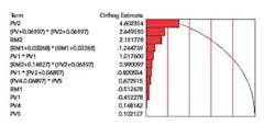
A Pareto of Effects chart (Figure 1) lists the variables in the model in decreasing order of significance, with the terms near the top of the list having the highest impact on the measured response “dissolution”. The Pareto made it clear that Process Variable 2 (PV2) and its squared terms were dominating the model.
Figure 1. Pareto of Effects for Final Model
A prediction profiler (Figure 2) provides a visual representation of the relationship among the significant variables, which have been narrowed to six: RM 1 and 2; and PV 1, 2, 4 and 5. The other three variables have been screened out. Again, it’s clear from the slope of PV2, which expresses the relative effect of that variable on the measured response, that PV2 has a major impact on dissolution, while such factors as PV4 and PV5 have far less impact.
Figure 2. Prediction Profiler for Final Model (With Optimum Settings)
Understanding the Design Space
Although PV2 exerts the greatest influence on dissolution, it is clear from the results of the DoE that other process and raw material variables and their interactions also play a role. The various permutations of the settings for the all of these variables that still result in an in-spec rate of dissolution (and other product properties) may be conceived of as the design space for the manufacture of the product.
To arrive at a better picture of the technologic space and to understand the design space in which to operate, a “Contour Profiler Matrix Plot” (Figure 3) was created using the optimum settings for each of the six significant variables. This tool brings together 15 three-dimensional response surface plots, each of which was originally created in the modeling software. The X and Y axes are made up of the DoE variables, and the Z axis (the contour curves) represents dissolution (the response variable). In the red regions, dissolution is out of specification and in the green regions it is within specification.
Figure 3. Contour Matrix Plot for Final Model
Each of the cells is a three-dimensional plot in which the “Y” variable is to the left of the cell, the “X” variable is below the cell, and the “Z” variable is the measured response, dissolution. For example, the top left cell has RM1 as the “Y” axis, RM2 as the “X” axis, and the surface depicted within the plot represents the dissolution.
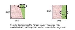
The goal is to find an available design space in which PV2 – by far the most influential variable – interacting with other variables can produce in-specification dissolution. That is: what values for PV2, along with what values for the other variables, offer the optimum path to achieving the desired rate of dissolution? In order to optimize this process (and stay “in the green”), the PV2 variable needs to be kept at a high level. Whenever the PV2 variable is low, the dissolution is out of specification. Concurrently, in order to maximize the “green space,” the RM2 variable should be maximized, and the RM1 variable should be kept in the center of the range used (see Figure 4).
Figure 4. Maximizing the Green Space
Confirming the Results
When the optimum conditions were entered into the model, the predicted dissolution rate was 49.7% after eight hours, almost right in the middle of the in-specification range of 40-60%. To confirm these predicted results and validate the final DoE model, two confirmation batches were processed as closely as possible to the optimum conditions that had been determined by the regression model and depicted in the Contour Profiler Matrix Plot.
The Outcome
Due to raw-material constraints, regulatory constraints, and processing constraints, the final settings that were utilized for the confirmation batches deviated slightly from the optimum conditions. The model prediction and confidence interval were 49.7 and 45.2 to 54.2, respectively. The results of the confirmation trials fell within the established confidence interval, thus confirming the validity of the model. The company then began looking more deeply into the variables that were identified in this study, particularly PV2 and RM2. Using the parameters that were optimized in the course of the study, the company successfully validated and launched the product.
Taking Advantage of Greater Regulatory Space
This study uncovered the critical interactions between process variables and raw material variables. Instead of running the process at a constant, pre-defined value of PV2, the design space prescribes adjusting PV2 based upon prior information known about RM1 and RM2, a far more successful approach.
By successfully defining the design space for a product, a company can open up more regulatory space under ICH Q8. Because they fully understand the various permutations of input variables and process parameters that could assure an in-specification product, the company can gain far more flexibility in changing process parameters and other variables. For example, when raw material batches vary, the company can make the necessary adjustments in the manufacturing process to compensate for the effects of differing properties and be confident that the resulting product will meet specifications. Within the design space, they can also continue to optimize and improve their manufacturing operation without facing additional regulatory filings or scrutiny.
Toward Long-Term Advantage
Most importantly, companies that master the concepts of technologic, design, and regulatory space can transfer that understanding to drug development and manufacturing throughout their operations, and thereby gain significant business benefits. The fewer deviations and rejected batches that result from greater operating flexibility reduces costs and ensures a reliable stream of supply to the market. A lightened regulatory burden and greater confidence in the ability to maintain in-specification operations frees resources for more productive investment. In short, the companies that win this space race will win on the bottom line and in the marketplace.
About the Author
Jason Kamm is a managing consultant with Tunnell Consulting, located in King of Prussia, Pa. He can be reached at [email protected] or at (610) 337-0820.
Reference
“ICH Harmonized Tripartite Guideline: Pharmaceutical Development, Q8,” Current Step 4 Version, November 10, 2005, p. 11.


