[Editor’s note: This article was originally published on the Lean Labor Strategies site. Permission to repost here has been granted by the author.]
Ask a manufacturing engineer or production supervisor how long they have been under pressure to reduce costs and improving productivity and they’ll most likely say since they started working.
Improvement methodologies such as Total Quality Management and Design for Manufacturability come on strong and manufacturers rally around them as a new approach to wringing incremental performance out of operations. And yet decades later on the production floor, some weeks everything performs flawlessly and other weeks it seems that Murphy’s extended family has come to visit.
Fatigue with the improvement projects can set in over the years because the big issues of a production line have been managed. The machines are rarely down for more than an hour. Kanbans to manage and reduce WIP have been implemented. As the teams move down the Pareto chart, the big gains have been achieved and each new effort seems to return less gain. Eventually people move on to other issues and performance of the production line flattens out.
Chasing down the biggest issues first is so ingrained in our minds that it seems almost like a law of nature. Invoking a justification of Pareto analysis, commonly known as the 80/20 rule brings nods of agreement in justifying the order of how issues should be addressed.
But there is a follow up question that should be asked that almost never is: “Even though we’ll solve our biggest issue, how much variability will be left in our system based on the remaining issues.”
This is an important question because the process will suffer from the cumulative effects of the remaining variability. The workforce can be a significant cause of variability. So as the number of employees that participate in the process increase there is going to be a cumulative effect of variability from each employee within the overall process.
This is supported by statistical analysis which will be described shortly, but for those not familiar with statistics, a more familiar way of explaining this would be as follows:
Let’s say we wanted to meet a co-worker after work at a restaurant to celebrate an event. If we invite one person, we can be fairly certain they will be there on time. But as we increase the number of co-workers invited, it becomes increasingly likely that some will be late. A few will have last minute calls from customers; others will be stuck in meetings that run over. And others will have emergencies at home that require their immediate attention.
The same happens in production; as the number of people increase within a process, the inevitable delays that occur increases as the number of people increase. Without directly managing all the little issues that cause this delay for each individual, there’s a limit to the amount of improvement that can be achieved in production.
But compared to a celebratory night out after work where only 2 people need arrive to begin the party, in manufacturing, everyone has to show to begin working.
Statistical analysis can be used to describe this scenario and even predict the variability and delay. The cumulative effect of the delays can be expressed as what is commonly referred to as the Sum of Independent Variables. Statistics show that the means (average) and variances of multiple independent variables are cumulative.
As each employee is an independent variable, their effect in terms of delay on production is cumulative. In order to bring a process into control requires the management of all the independent variables affecting the process including the workforce.
This can be described through a manufacturing example as well. Disruptions are considered when an operation is completed sooner or later than expected.
In this example, the process has been in place for years and the big issues causing disruptions have been resolved. For the most part the equipment is never down for more than a couple of hours and material quality and dimensional issues have been ironed out. The labor standard that is used to measure, cost and schedule the process is now a reflection of the actual average time it takes to complete this process.
To begin with, the example starts out very simply. There is one person on the line. This defines N (N equals the number of independent variables or people in this case) as equal to 1.
Experience would tell us that most days the process goes as planned. Almost nothing happens out of the ordinary and production runs as expected. Here are some examples of the disruptions that do occasionally occur in this process.
- While typically punctual, a couple of times a month an operator is late getting into work and production starts behind schedule.
- Skill levels vary between operators and they complete an operation in slightly different amounts of time.
- The operator is delayed by others such as a maintenance person or material handler
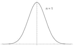
The curve below describes an example of the frequency and impact of those events; it’s a familiar shape and known in statistics as a Gaussian distribution or normal curve. For the purpose of this example the average time (or labor standard) to complete this operation is 2 hours for N=1. The variance in production time this example has been measured at 30 minutes, but the curve could apply to any cycle time and variance.
Variance = б² = 30 minutes
To make the example more typical of an actual production scenario, 14 more operators and operations are added to the process. Each one of these people is considered an independent variable. As stated above in the discussion of the Sum of Independent Variables, the mean and variance of the delays that each person causes are cumulative. Now N (Number of independent variables) = 15.
The average production cycle time is:
Mean = N * μ = 15 * 2 = 30 hours
Variance = N * б² = 15 * 30 = 450 minutes = 7.5 hours
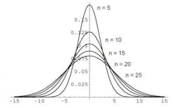
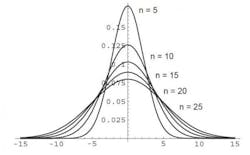
When the independent variable ( a production operator in this case) has a Gaussian distribution, the distribution of the sum is also Gaussian. The graph below shows how the distribution broadens as N is increased. For convenience of graphing, the mean is set to zero. Obviously with a non-zero mean, the distributions would also shift to the right of the graph. In other words, the mean for one person is two hours, the mean for 15 people is 30 hours, in this case all distributions are set at 0.
Distribution of variance in time as the number of people and operations in a process changes (N=5,10,15 or 20 people)
With N=1 person, the variation in work time is relatively small, centered around the standard work interval of 2 hours. With N=10 or 15 people, it seems like almost every day there is some event occurring. Between machine jams, operators calling in sick, temporary help on the line due to turnover and maintenance mechanics who are busy working on other equipment, the variations in performance add up over the course of a month. Every once in a great while, it seems like nothing goes right and hours of production are lost. This cumulative effect is reflected in the Gaussian distribution with N=15 in the figure above. The variations in the total production time are significantly greater than one might expect by intuitively extrapolating from one operator to 15.
Because these individual delays are typically small, it feels like they are unmanageable or that investing in solving all the different causes would not justify the returns. However there is a difference between managing production equipment and individuals. Controlling each piece of capital equipment, while similar, requires a different approach due to their unique design of tooling, dies and capacity. Individuals, while also unique, all respond well to equitable and fair management. This means the investment required to decrease labor related delays on production can be spread across all operators and support staff on the line. Additionally, it affects the operators and support staff on all production lines. The result is instead of working down the workforce related variables one person at a time, the workforce as a whole improves providing significant improvement. In this example, the improvements reduce delays.
To understand the return on investment possible, if the disruptions to the operation due to labor is reduced by 10% the variance of the operation is reduced by 45 minutes.
The result is production schedule adherence improves, and the need for overtime decreases, idle time in downstream operation is reduced and costs such as premium freight and inventory buffers are reduced as well.
As one of the three pillars of Lean, the workforce has long been recognized as critical to the success of operation. But in practice, because an individual’s impact on an entire operation in terms of delay can be small, managing the individual is often moved down in priority. Experienced Lean practitioners may suggest these small variances are why self empowerment is important. But viewing the cumulative impact of small variances across an entire production team and supporting staff is something an individual can’t see. The value of the effort is found in identifying and systematically managing common, small variance across the entire workforce.


